Examples
This page show examples of COMPS in action.
Neighbourhoods for precipitation
High-resolution models often produce realistic looking precipitation patterns, although the exact placement of individual showers can have little skill. To account for uncertainty in placement, each grid point can be smoothed by averaging all grid points within a neighbourhood.
Figures (a), (b), and (c) show the gridded field after the neighbourhood approach has been applied separately to each grid point. 3 different neighbourhood sizes are used.
When topographic forcing is present, smoothing removes the elevation gradient that may actually be modelled correctly. To maintain the elevation gradient while allowing the field to be sufficiently smoothed, we can use a neighbourhood method that uses only neighbouring grid points that are at a similar elevation (d).
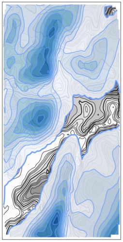
(a) Nearest neighbour
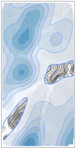
(b) Nearest 36 neighbours
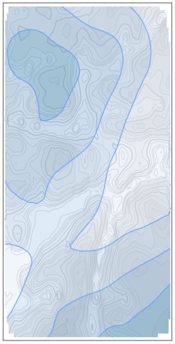
(c) Nearest 225 neighbours
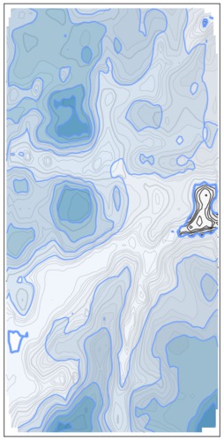
(d) Nearest 100 "same-elevation" neighbours
Bias-correction of temperature
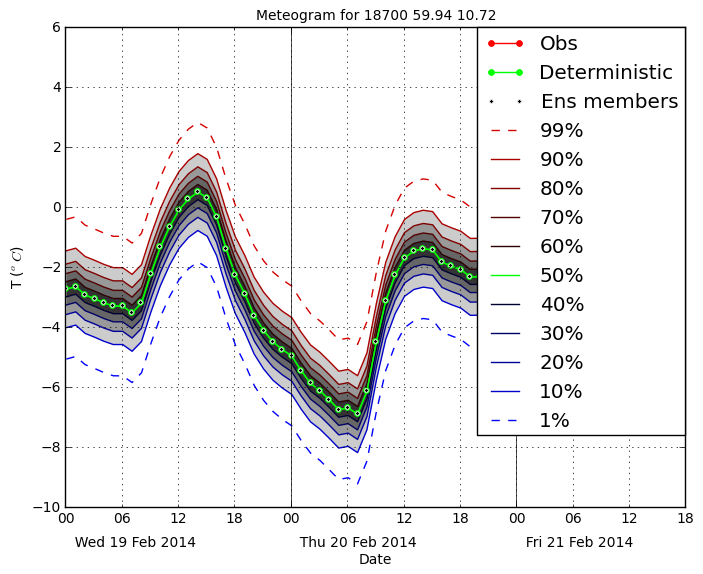
Raw forecast

Kalman filtered forecast